Linear Regression

Formula

#

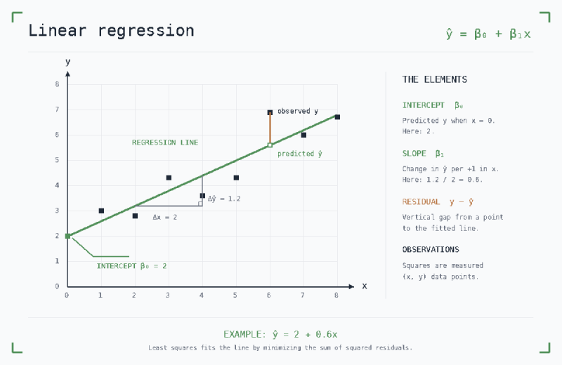
When using Linear Regression, the goal is to estimate a function $f(x)$ such that each feature has a linear relationship to the target variable $y$.
This is a supervised learning model written as:

$$ y = \beta_0 + X\beta $$

with:

• $\beta_0$ = intercept (or bias)
• $X$ = matrix of predictor variables
• $\beta$ = vector of parameters that determine the weights for each variable. For a single predictor, the sign of $\beta$ gives the direction of the relationship:
  • $\beta > 0$ is positive
  • $\beta < 0$ is negative
  • $\beta = 0$ means no linear effect.

Estimation framework

#

The Ordinary Least Squares (OLS) sets the objective to find a straight line that passes as close as possible to all data points simultaneously, looking at the residuals for defining closeness.

Loss function

#

Linear regression estimates the weights $\beta$ by minimizing the Residual Sum of Squares (RSS).

Optimization

#

The (RSS) minimization typically happens using gradient descent (if the dataset has many features) or normal equation (if the dataset is small enough to compute matrix inverses).

Evaluation

#

A popular metric for assessing its goodness is R squared. Other error metrics to measure linear regression goodness are:

• mean squared error(MSE)
• mean absolute error(MAE)

Algorithm

#

The training process is about learning the model weights \(\beta\):

1. The dataset contains multiple rows of labeled values $(y, x_1, x_2, \ldots, x_n)$. The linear formula for predicting $y$ is $$\tilde{y} = \beta_0 + \beta_1x_1 + \beta_2x_2 + \ldots + \beta_nx_n$$
2. Initialize the weights, \(\beta\), to random values
3. Compute \(\tilde{y}\) for each row
4. Compute the loss for each row as \((y - \tilde{y})^2\) (squared loss). Other losses are possible such as absolute value difference, \(\lvert y - \tilde{y} \rvert\), or a weighted combination of quadratic and absolute value. Additionally, we typically add a regularization term to the loss value. The loss value is used to determine if we have converged (see step 8).
5. Compute the gradient of loss with respect to each parameter :
   • Gradient of loss with respect to \(\beta_0\) is \(2(y - \tilde{y})(-1)\)
   • Gradient of loss with respect to \(\beta_k\) is \(2(y - \tilde{y})(-x_k)\)
6. Update each of the weights by their gradients: \(\beta_k := \beta_k - \eta(y - \tilde{y})x_k\), where \(\eta\) is a single global learning rate hyperparameter
7. Repeat steps 3 to 6 until convergence, or until average loss over datapoints is less than a predefined tolerance or error rate, or for a certain number of repetitions (epochs) of the algorithm

The numpy implementation of the algorithm above is in Linear Regression from scratch.

Assumptions

#

• Linearity: the relationship between the features set and the target is linear
• Homoscedasticity: the variance of the residuals is constant
• Independence: all observations are independent of one another
• Normality: the distribution of \(y\) is assumed to be normal

If these assumptions are violated, any forecast or confidence interval based on the model will likely be misleading or biased.

Pitfalls

#

• Heteroscedasticity: this is the opposite of homoscedasticity, where the variance of the residuals is not constant, and the residuals are not identically distributed.
• Residuals distribution non-normality
• Outliers
• Multicollinearity: predictors are correlated and affect the resulting coefficients estimate.