
Batch size refers to the number of training examples processed in a batch, which corresponds to a single forward pass and backward pass before the model updates its weights.
For instance, if a dataset contains 10,000 images and the batch size is set to 64, the model splits the dataset into subsets of 64 images, calculates the average error (loss) across those 64 samples, updates its weights, and then moves to the next batch.
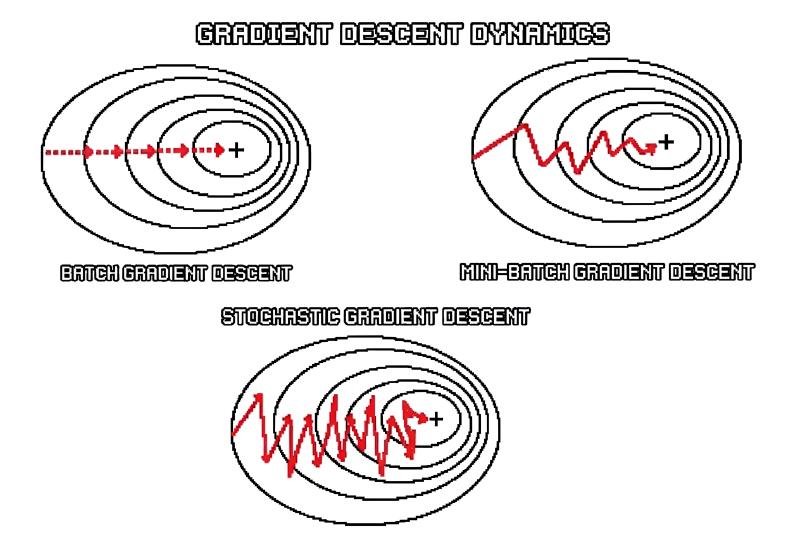
The path a model takes toward optimal weights changes drastically depending on the batch size:
- Stochastic (Batch Size = 1): Updates weights after every single sample. The gradient trajectory is noisy and erratic, making frequent directional changes.
- Full-Batch (Batch Size = Total Dataset Size): Computes gradients using the entire dataset for a single update. The trajectory is direct and smooth toward the nearest minimum.
- Mini-Batch (Batch Size = 32, 64, 128, etc.): A middle ground that combines stability with noisy gradient updates.
Implications: Small vs. Large Batch Size#
Small Batch Size (e.g., 8, 16, 32)#
Advantages:
- Better Generalization: The noise introduced by smaller samples acts as a implicit regularizer, preventing the model from overfitting and helping it escape sharp local minima toward flatter, more stable minima.
- Low Memory Footprint: Requires significantly less GPU/VRAM memory per iteration.
- Faster Early Convergence: Frequent weight updates mean the model starts learning immediately without waiting to process large volumes of data.
Disadvantages:
- Hardware Inefficiency: Modern GPUs excel at parallel computation; small batches leave matrix multiplication units (e.g., Tensor Cores) underutilized.
- Noisy Training Dynamics: High gradient variance can lead to unstable loss curves or divergence if the learning rate is too high.
Large Batch Size (e.g., 512, 1024, 8192+)#
- Advantages:
- High Hardware Throughput: Maximizes GPU/TPU parallel utilization, drastically speeding up total epoch training time.
- Accurate Gradient Estimates: The calculated gradient closely mirrors the true population gradient, resulting in stable, smooth convergence.
- Disadvantages:
- Generalization Gap: Large batches tend to converge into sharp local minima, leading to worse performance on unseen test data compared to smaller batches.
- High Memory Consumption: Can quickly result in Out of Memory (OOM) errors, especially with large architectures (e.g., LLMs, high-resolution Vision transformers).
- Requires hyperparameter Scaling: Often demands a corresponding increase in learning rate (e.g., using linear scaling rules) or warm-up schedules to avoid early training stagnation.